%matplotlib inline
import matplotlib.pyplot as plt
import numpy as np
import sympy as sy
from math import atan2

Visualizing Differential Equations

Returning to the example from our last notebook, we had the differential equation

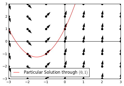
\[\frac{dy}{dx} = 2x + 3\]

Interpreting this geometrically we are looking at a relationship where the slope of the tangent line at some point \((x,y)\) is given by \(2x+3\). For example, at any point where \(x = 1\), we have the slope of the tangent line equal to \(2(1) + 3 = 5\). We can draw a small short line at each of these points to represent this behavior. Similarly, we could repeat this for a small number of \(x\) and \(y\) values. Most important, is that we understand we are not finding a single line solution, but rather representing tangent lines of a family of functions just like our initial general solutions to the ODE.

def dy_dx(x):
    return 2*x + 3

x = np.arange(-3,4, 1)
y = np.arange(-3,4, 1)
X,Y = np.meshgrid(x, y)

X

array([[-3, -2, -1,  0,  1,  2,  3],
       [-3, -2, -1,  0,  1,  2,  3],
       [-3, -2, -1,  0,  1,  2,  3],
       [-3, -2, -1,  0,  1,  2,  3],
       [-3, -2, -1,  0,  1,  2,  3],
       [-3, -2, -1,  0,  1,  2,  3],
       [-3, -2, -1,  0,  1,  2,  3]])

Y

array([[-3, -3, -3, -3, -3, -3, -3],
       [-2, -2, -2, -2, -2, -2, -2],
       [-1, -1, -1, -1, -1, -1, -1],
       [ 0,  0,  0,  0,  0,  0,  0],
       [ 1,  1,  1,  1,  1,  1,  1],
       [ 2,  2,  2,  2,  2,  2,  2],
       [ 3,  3,  3,  3,  3,  3,  3]])

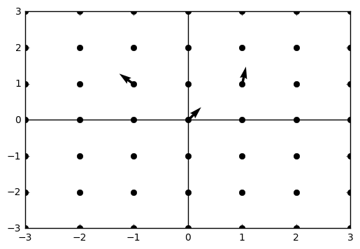
fig = plt.figure()
plt.plot(X,Y, 'o', color = 'black', markersize = 6)
plt.axhline(color = 'black')
plt.axvline(color = 'black')
ax = fig.add_subplot(111)
ax.quiver(0,0,2,2)
ax.quiver(1,1,1.1,2*(1.1) + 3)
ax.quiver(-1,1,-1.1, 2*(-1.1) + 3)

<matplotlib.quiver.Quiver at 0x11fcd9160>

atan2(dy_dx(2), 1)

1.4288992721907328

theta = [atan2(dy_dx(i), 1) for i in x]

theta

[-1.2490457723982544,
 -0.7853981633974483,
 0.7853981633974483,
 1.2490457723982544,
 1.373400766945016,
 1.4288992721907328,
 1.460139105621001]

plt.quiver(X,Y, np.cos(theta), np.sin(theta))
plt.axhline(color = 'black')
plt.axvline(color = 'black')
plt.plot(X, Y, 'o', color = 'black')
x2 = np.linspace(-3,3,1000)
plt.plot(x2, x2**2 + 3*x2 + 1, '-k', color = 'red', label = 'Particular Solution through $(0,1)$')
plt.xlim(-3,3)
plt.ylim(-3,3)
plt.legend(loc = 'best')

<matplotlib.legend.Legend at 0x120e02438>