In [2]:
%matplotlib inline
import matplotlib.pyplot as plt
import numpy as np
import sympy as sy
Parametric Descriptions
To this point, we have primarily seen relationships between quantities expressed in explicit terms of one another. In other words we usually have something like \(y=\) or \(x =\), with the other side of the expression having expressions in terms of another variable.
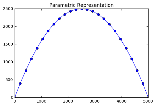
Alternatively, we can describe the relationships between quantities in terms of their value at some additional parameter. The example of displacement of a projectile body is a sensible example, where you would want to know the position of the particle at some time \(t\). For this, we have an expression for both the \(x\) and \(y\) coordinates of the body in terms of some time \(t\) for \(0\leq t \leq 25\).
We can plot this in Python by defining the values of \(t\) and functions \(x(t)\) and \(y(t)\) as usual.
This also means, for example, that at time \(t=5\), the body is located at \((1000, 1600)\).
In [3]:
t = np.linspace(0, 25, 25)
def x(t):
    return 200*t
def y(t):
    return 400*t - 16*t**2
In [4]:
plt.plot(x(t), y(t), '-o')
plt.ylim(0, 2500)
plt.xlim(0,5000)
plt.title("Parametric Representation")
Out[4]:
<matplotlib.text.Text at 0x10e73cba8>
Calculus on Parametrically Defined Functions
We can operate on the expressions as we had earlier. Now, we are describing the rate of change independently in the \(x\) and \(y\) direction in terms of a unit of time \(t\). Consider two points \(P_0 = (x(0), y(0))\) and \(P_1 = (x(1), y(1))\).
The change in \(x\) would be given by \(x_1 - x_0\). The change in \(y\) would be found with \(y_1 - y_0\), just as we have seen before. This is simple because we are using time intervals of 1, however just like before we can imagine that shrinking these to infinitely small intervals gives us a derivative in terms of \(t\). Recall our earlier description of the tangent as:
Sympy allows us to find all of these derivatives easily.
In [5]:
x, y, t = sy.symbols('x y t')

def x(t):
    return 200*t
def y(t):
    return 400*t - 16*t**2
In [6]:
dxt = sy.diff(x(t), t)
In [7]:
dyt = sy.diff(y(t), t)
In [8]:
dydx = dyt/dxt
dydx
Out[8]:
-4*t/25 + 2
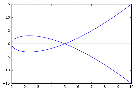
Tangent Lines
In [9]:
t = np.linspace(-3,3, 100)

def x(t):
    return t**2 + 1
def y(t):
    return t**3 - 4*t

plt.plot(x(t), y(t))
plt.axhline(color = 'black')
Out[9]:
<matplotlib.lines.Line2D at 0x10e730c50>
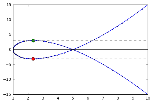
In [10]:
x, y, t = sy.symbols('x y t')

def x(t):
    return t**2 + 1
def y(t):
    return t**3 - 4*t
In [11]:
dx = sy.diff(x(t), t)
dy = sy.diff(y(t), t)
eq = dy/dx
In [12]:
a, b = sy.solve(eq)
In [13]:
t = np.linspace(-3,3, 100)
def x(t):
    return t**2 + 1
def y(t):
    return t**3 - 4*t


plt.plot(x(t), y(t), '-o', markersize = 2)
plt.plot(x(a), y(a), 'o', markersize = 8)
plt.plot(x(b), y(b), 'o', markersize = 8)
plt.axhline(color = 'black')
plt.axhline(y(a), ls = '--', color = 'grey')
plt.axhline(y(b), ls = '--', color = 'grey')
Out[13]:
<matplotlib.lines.Line2D at 0x10ee5df60>
Additional Examples
Some additional examples of parametric curves are as follows:
Line: Through point \((a, b)\) with slope \(m\) \(\rightarrow c(t) = (a + t, b + mt)\)
Circle: Radius \(r\) centered at \((a, b)\) \(\rightarrow x(\theta) = a + r\cos(\theta) \quad y(\theta) = b + r\sin(\theta)\)
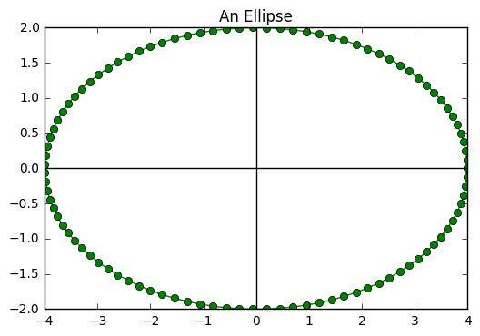
Ellipse: An ellipse of the form \((\frac{x}{a})^2+ (\frac{y}{b})^2 = 1\) is parameterized by \(\rightarrow c(t) = (a\cos(t), b\sin(t))\)
In [14]:
t = np.linspace(0, np.pi*2, 100)

x = 4*np.cos(t)
y = 2*np.sin(t)


plt.plot(x, y, '-o', c = 'green')
plt.xlim(min(x), max(x))
plt.ylim(min(y), max(y))
plt.title("An Ellipse")
plt.axhline(color = 'black')
plt.axvline(color = 'black')
Out[14]:
<matplotlib.lines.Line2D at 0x10ef9cbe0>
In [15]:
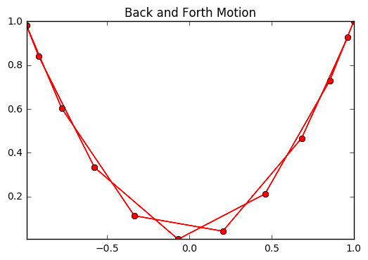
t = np.linspace(0, np.pi*4, 24)
x = np.cos(t)
y = np.cos(t)**2
plt.plot(x, y, '-o', c = 'red')
plt.xlim(min(x), max(x))
plt.ylim(min(y), max(y))
plt.title("Back and Forth Motion")
Out[15]:
<matplotlib.text.Text at 0x10eff39b0>
In [16]:
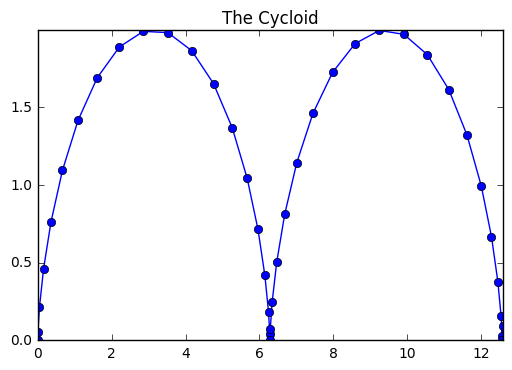
t = np.linspace(0, 13, 40)
x = t - np.sin(t)
y = 1 - np.cos(t)

plt.plot(x, y, '-o')
plt.xlim(min(x), max(x))
plt.ylim(min(y), max(y))
plt.title("The Cycloid")
Out[16]:
<matplotlib.text.Text at 0x10f115358>
Problems
Interpolation
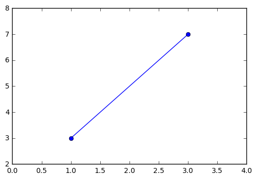
Let’s suppose we have two points, defined parametrically, \(P_0 = (1, 3)\) and \(P_1 = (3, 7)\). Suppose also, that we have a body in motion between the points. This body at time \(t=0\) is at \(P_0\) and at time \(t=1\) is at \(P_1\). We can intuit the parametric equations for \(x(t)\) and \(y(t)\) as:
The plot below demonstrates the simple situation.
In [16]:
x = [1, 3]
y = [3, 7]
plt.plot(x, y, '-o')
plt.xlim(min(x)-1, max(x)+1)
plt.ylim(min(y)-1, max(y)+1)
Out[16]:
(2, 8)
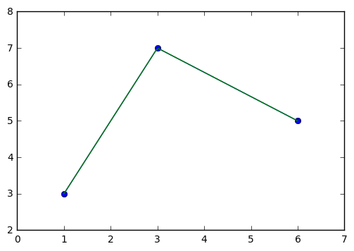
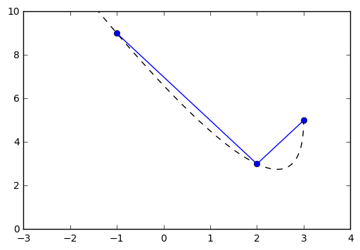
We can extend the problem to three points as follows. Further, we can use numpy to interpolate the segments. To do so, we need to describe the interval of \(x\) values that we want to interpolate the curve. Here, we start at \(x = 1\) and end at \(x = 6\).
In [53]:
x = np.linspace(1, 6, 100)
xs = [1, 3, 6]
ys = [3, 7, 5]
plt.plot(xs, ys, '-o')
curve = np.interp(x, xs, ys)
plt.plot(x, curve)
plt.xlim(min(xs)-1, max(xs)+1)
plt.ylim(min(ys)-1, max(ys)+1)
Out[53]:
(2, 8)
If we consider the same problem for any two points \((x_0, y_0), (x_1, y_1)\) we would have:
and more generally in terms of the points \(P_0\) and \(P_1\) we have
We can hypothesize that this relationship would hold true for further points. For example, if we add a third point \(P_2\) it seems reasonable to expect that we would have an expression combining these points with some functions \(\alpha(t)\) as follows.
We can extend the problem above and again determine that equal time intervals will be traversed between each pair of points, and that at time \(t = 0, 1, 2\) we are at points \(P_0, P_1, P_2\) respectively to form a polynomial.
EXAMPLE: Suppose we now take points \(P_0 = (-1,9), P_1 = (2, 3), P_2 = (3, 5)\). Thus \(\alpha_0(0) = 1, \alpha_0(1) = 0, \alpha_0(2) = 0\). If we assume that the curve passing through these points is only zero at \(t = 1, 2\) we have \(\alpha_0(t) = a(t - 1)(t - 2)\) for some \(a\), but we also know that at \(\alpha_0(0) = 1\) so
Through similar procedures verify that \(\alpha_1(t) = -t(t-2)\) and \(\alpha_2(t) = \frac{t(t-1)}{2}\), or
which gives
In [86]:
def x(t):
    return -t**2 + 4*t -1
def y(t):
    return 4*t**2 - 10*t + 9
t = np.linspace(-2,2,100)
P = [-1,2,3]
Y = [9, 3, 5]

plt.plot(x(t), y(t), '--k')

plt.plot(P, Y, '-o')
plt.xlim(-3,4)
plt.ylim(0,10)
Out[86]:
(0, 10)
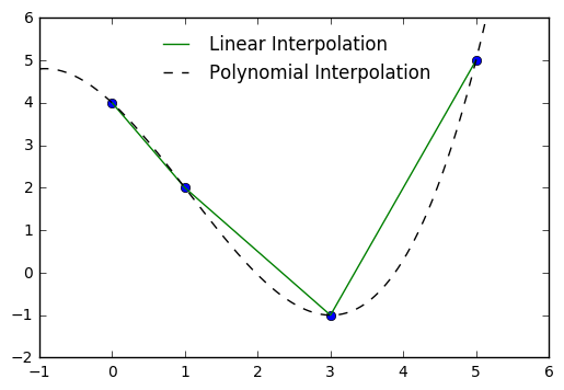
And with four points we have a similar example, where we now use the
scipy.interpolate function.
In [62]:
x = [0, 1, 3, 5]
y = [4, 2, -1, 5]
curve = np.interp(x, x, y)
In [65]:
from scipy import interpolate

i1 = interpolate.splrep(x, y, s=0)
ynews = interpolate.splev(xs, i1, der = 0)

plt.plot(x, y, 'o')
plt.plot(x, curve, label = "Linear Interpolation")
plt.plot(xs, ynews, '--k', label = "Polynomial Interpolation")
plt.xlim(min(x)-1, max(x)+1)
plt.ylim(min(y)-1, max(y)+1)
plt.legend(loc = 'best', frameon = False)
Out[65]:
<matplotlib.legend.Legend at 0x119b6a208>
Bezier Curves
A variant of the problem of interpolating polynomials is the use of computer graphics programs to manipulate a curve. This is the problem that him and him encountered as engineers in for automotive manufacturers in the 1960’s. The idea, rather than finding the interpolating polynomial, is to form a polynomial contained withing the framework of the linear piecewise image.
For example, we can create a simple quadratic with two sections similar to our earlier shapes. Now, suppose we have a point affixed on each of these sections joined by a bar. Also, suppose these points traverse the distance between successive vertices in equal time. We can trace out a simple quadratic by following the point \(P\) as the bar moves.
In [87]:
x = [1, 3, 6]
y = [1, 5, 4]
plt.figure(figsize = (10,6))
plt.plot(x, y, '-o')
plt.plot((x[0]+x[1])/2, (y[0]+y[1])/2, '-o')
plt.plot((x[1]+x[2])/2, (y[1]+y[2])/2, 'o')
plt.xlim(min(x)-1, max(x)+1)
plt.ylim(min(y)-1, max(y)+1)
plt.annotate('$P_0$', xy = (x[0]-0.5, y[0]))
plt.annotate('$P_1$', xy = (x[1]-0.5, y[1]))
plt.annotate('$P_2$', xy = (x[2]-0.5, y[2]+0.5))
plt.annotate('$P_{01}$', xy = ((x[0]+x[1])/2 - 0.4, (y[0]+y[1])/2))
plt.annotate('$P_{12}$', xy = ((x[2]+x[1])/2 - 0.4, (y[2]+y[1])/2 + 0.3))
a = [(x[0]+x[1])/2, (x[1]+x[2])/2]
b = [(y[0]+y[1])/2, (y[1]+y[2])/2]
plt.plot(a, b, color = 'blue')
plt.plot((a[0]+a[1])/2, (b[0]+b[1])/2, 'o')
plt.annotate('$P$', xy = ((a[0]+a[1])/2, (b[0]+b[1])/2+.2))
plt.title("A Simple Bezier Spline Generated by Point $P$")


bez = [x[0], (a[0]+a[1])/2, x[2]]
bezy = [y[0], (b[0]+b[1])/2, y[2]]
i1 = interpolate.interp1d(bez, bezy, kind = 'quadratic')
xs = np.linspace(1, 6, 1000)
plt.plot(xs, i1(xs), '--k')
Out[87]:
[<matplotlib.lines.Line2D at 0x11938e630>]
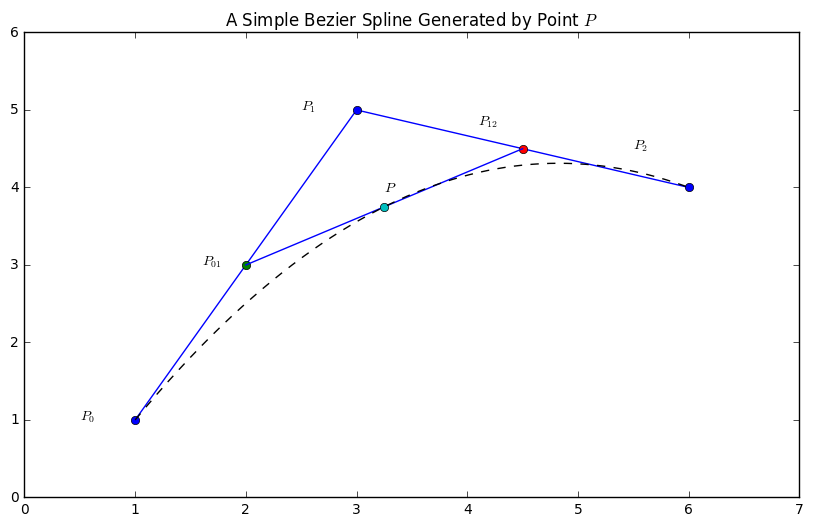
The Bezier quadratic is given by the function \(P(t)\) as \(t\) goes from 0 to 1. It takes the form:
or parametrically as