Measuring Cardiac Output: Turkeys on Treadymills
GOALS:
- Connect Summations to Cardiac Output problems
- Use summations to solve problems from biology
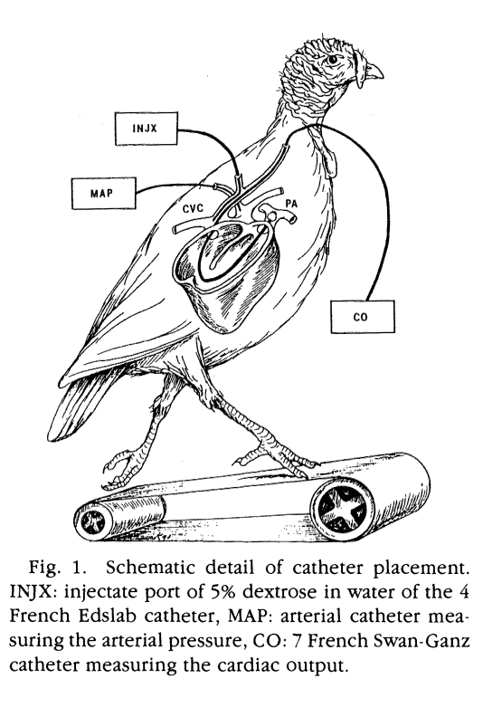
This notebook applies our techniques for area approximation to the problem of measuring Cardiac Output. This is a measure of how fast the heart is circulating blood, and has obvious important consequences for humans and animals. The image below comes from a study on the cardiac output of Turkeys.
Dye Dillution Method
The main idea of the Dye Dillution method is to inject dye into a subjects blood, and measure how much of the dye flows through the heart over small time intervals. From Wikipedia.
The dye dilution method is done by rapidly injecting a dye, indocyanine green, into the right atrium of the heart. The dye flows with the blood into the aorta. A probe is inserted into the aorta to measure the concentration of the dye leaving the heart at equal time intervals [0, T] until the dye has cleared. Let c(t) be the concentration of the dye at time t. By dividing the time intervals from [0, T] into subintervals Δt...
In the example of the Turkey on the Treadmill, a device was implanted to monitor the dispersion of dye in the Turkey while running on a treadmill. This could then be compared to Turkey’s hear rates who were relaxing in soft armchairs. This example comes from the study Effect of Exercis on Cardiac Output and Other Cardiovascular Parameters of Heavy Turkeys and Relevance to the Sudden Death Syndrome, by Boulianne, et al in the Journal of Avian Diseases, 37, 1993.
Example I
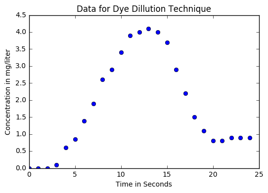
Imagine that we have the following data on dye concentration over the course of 26 seconds. The intervals are equal at 1 second. Let’s create two lists for the time intervals and the concentration measurements to plot them.
In [1]:
time = [i for i in range(25)]
In [2]:
concentration = [0, 0, 0, 0.1, 0.6, 0.85, 1.38, 1.9, 2.6, 2.9, 3.4, 3.9, 4.0, 4.1, 4.0, 3.7, 2.9, 2.2, 1.5, 1.1, 0.8, 0.8, 0.9, 0.9, 0.9]
In [3]:
%matplotlib inline
import matplotlib.pyplot as plt
import numpy as np
In [4]:
plt.plot(time, concentration, 'o')
plt.title("Data for Dye Dillution Technique")
plt.xlabel("Time in Seconds")
plt.ylabel("Concentration in mg/liter")
Out[4]:
<matplotlib.text.Text at 0x115fbeb38>
We can consider the cardiac output as the total volume of dye measured divided by the time as follows:
Similarly, we can express this as the amount of dye(D) over the volume(CT) as
Hence, in our example above, the \(CT\) is the sum of our list
concentration.
In [5]:
sum(concentration)
Out[5]:
45.42999999999999
Suppose, for example, that we injected 5 liters of dye in the example above. The cardiac output would be:
In [6]:
6/45.43
Out[6]:
0.13207131851199647
Or 0.1321 liters per second.
In [7]:
6/45.43*60
Out[7]:
7.924279110719788
7.9243 liters per minute.
Example II
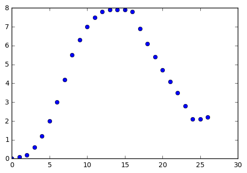
Suppose we have the following information about the flow of dye as follows. Find the cardiac output for this example.
In [8]:
t2 = [i for i in range(27)]
c2 = [0, 0.1, 0.2, 0.6, 1.2, 2.0, 3.0, 4.2, 5.5, 6.3, 7.0, 7.5, 7.8, 7.9, 7.9, 7.9, 7.8, 6.9, 6.1, 5.4, 4.7, 4.1, 3.5, 2.8, 2.1, 2.1, 2.2]
In [9]:
plt.plot(t2, c2, 'o')
Out[9]:
[<matplotlib.lines.Line2D at 0x118a1da58>]
Example III
The table below gives measurements after an injection of 5.5 mg of dye. The readings are given in mg/L.
| time | concentration in mg/L |
|---|---|
| 0 | 0.0 |
| 2 | 4.1 |
| 4 | 8.9 |
| 6 | 8.5 |
| 8 | 6.7 |
| 10 | 4.3 |
| 12 | 2.5 |
| 14 | 1.2 |
| 16 | 0.2 |
Example IV
The table below demonstrates a 6 mg injection of dye into a heart. Use the data to approximate the cardiac output. What kind of a creature could this be?
| time | concentration in mg/L |
|---|---|
| 0 | 0 |
| 2 | 1.9 |
| 4 | 3.3 |
| 6 | 5.1 |
| 8 | 7.6 |
| 10 | 7.1 |
| 12 | 5.8 |
| 14 | 4.7 |
| 16 | 3.3 |
| 18 | 2.1 |
| 20 | 1.1 |
| 22 | 0.5 |
| 24 | 0 |
Accounting for End Values
As we noticed in the examples, the monitor may return values towards the end of the readings that do not agree with our assumptions. In order to check this, we impose values that decrease on the end of the sequence. For example, in the list below, we change the final four values to better reflect the pattern we expect.
In [12]:
time = [i for i in range(25)]
concentration = [0, 0, 0, 0.1, 0.6, 0.85, 1.38, 1.9, 2.6, 2.9, 3.4, 3.9, 4.0, 4.1, 4.0, 3.7, 2.9, 2.2, 1.5, 1.1, 0.8, 0.8, 0.9, 0.9, 0.9]
%matplotlib notebook
import matplotlib.pyplot as plt
import numpy as np
In [13]:
plt.figure()
plt.plot(time[:21], concentration[:21], 'o')
plt.plot(time[21:], concentration[21:], 'ro', label='Readings for Last Values')
plt.title("Data for Dye Dillution Technique")
plt.xlabel("Time in Seconds")
plt.ylabel("Concentration in mg/liter")
plt.plot([21, 22, 23, 24], [0.4, 0.24, 0.14, 0.1], 'go', alpha=0.6, label = 'Approximations for Last Values')
plt.legend()

Out[13]:
<matplotlib.legend.Legend at 0x118b17860>