Introduction and Review¶

This notebook is meant to introduce the Jupyter notebooks and Python computing language and to show how they make solving many traditional mathematics problems easier. After getting started with the notebook, we run through some typical operations using python including variables, lists, plots, for loops, and functions. We demonstrate the use of these tools to solve some review mathematics problems from traditional Calculus textbook reviews.

Download and Start Jupyter¶

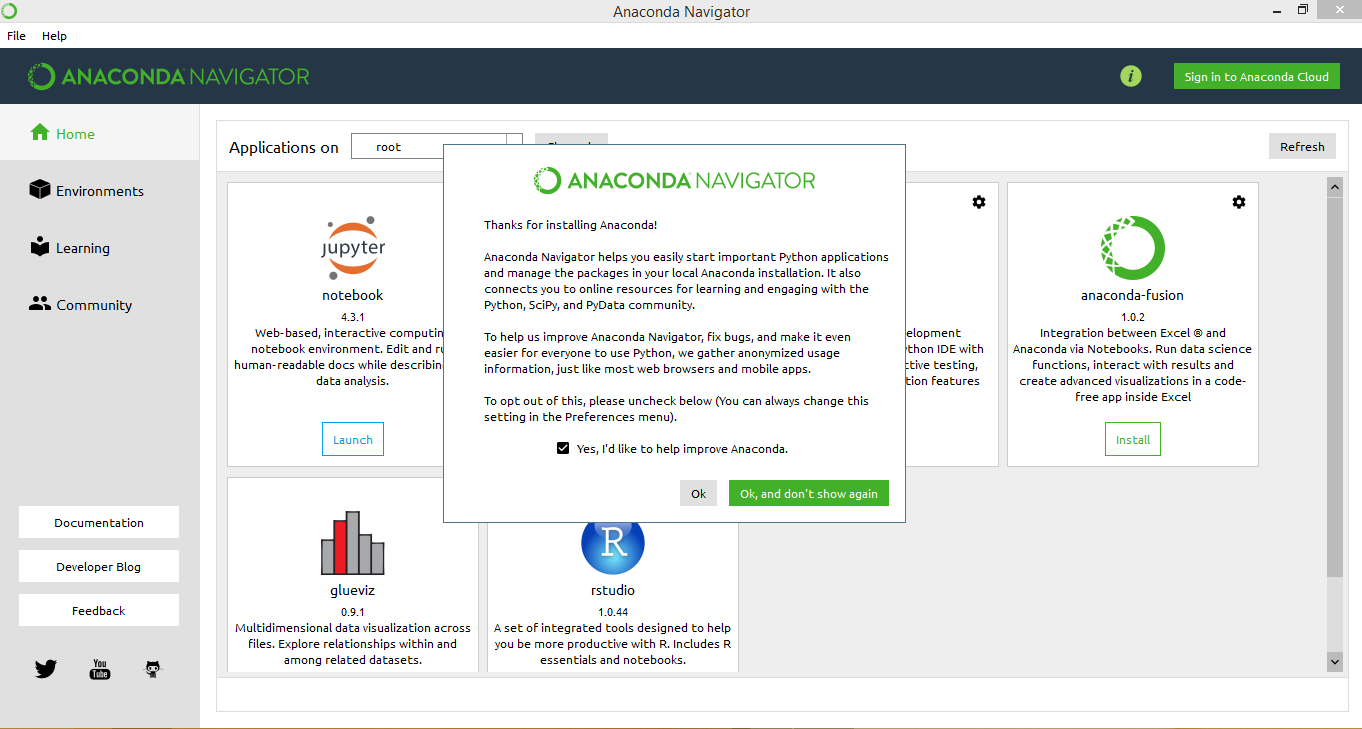
I recommend downloading and installing the most recent version of Anaconda available `here <>`__. You should choose the appropriate installation depending on your operating system. Once downloaded and installed, you can open the application and you should see something like the screen below.

Click on the Jupyter notebook tab and a browser window should open that has a file navigator similar to the image below.

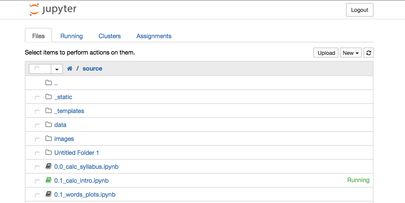
Add a new folder and rename it calc_notebooks. Now, you can go into this folder, and start a new Python 3 notebook.

Markdown Cells¶

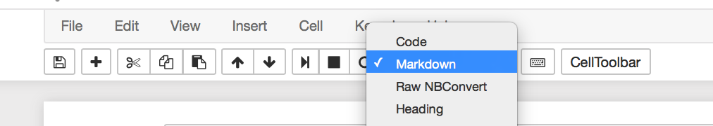
In your first notebook, you can click on the toolbar at the top and change the cell type. If you would like to type in a cell, we use a markdown cell. Markdown is a way to format typing with some minimal commands on the computer. Markdown cells also render many HTML tags, so if you are familiar with HTML you can use this to add effects to your documents.

Typing with Markdown¶

We use some simple syntax to create text effects in markdown. For example, to make a word bold we type **bold** and italics are a single asterisk *italics*. Sections can be denoted with different level headings using the # key as follows:

# Header I
## Header II
### Header III

Images with Markdown and HTML tags¶

Images can be added using simple markdown sytanx. Two things should be considered with images. First, I recommend storing them in a folder in the same directory as your notebooks. For example, I create a subfolder named images and place all my images there. For a larger project I will make image folders for each notebook.

The second important thing to remember is to use a continuous filename when saving the file. This means no spaces, i.e.

pig_pic.png not pig pic.png

From here, we use the markdown syntax

![](images/pig_pic.png)

to refer to an image in the folder images named pig pic. We can also use HTML image tags to show an image. Here, we can utilize some additional controls over the height and width of the image displayed. You can use some additional controls including the center and figure command to add a caption and center the figure on the page. This would be as follows:

<center>
<figure>
<img src = "pig_pic.png" height = 10 width = 20 >
<figcaption> This is a pig picture </figcaption>
</figure>
</center>

Python and Code Cells¶

To begin, we demonstrate the utility of Python as a calculator within code cells in Jupyter. The familiar arithmetic operations are as follows:

+ Addition
- Subtraction
* Multiplication
/ Division
** Exponentiation

To execute the cell, press shift + enter.

In [1]:

2 + 3

Out[1]:

In [2]:

1 + 3 * 5 * (2-4) - 7**2

Out[2]:

-78

In [3]:

1/2

Out[3]:

0.5

Types¶

There are different forms of information that Python understands. These types depend on the nature of the number or whether the entry is something other than a number like a string of symbols. We can investigate the type of an object using the type() function.

In [4]:

type(1), type(1/3), type("steve")

Out[4]:

(int, float, str)

In [5]:

a = 5

In [6]:

type(a)

Out[6]:

int

In [7]:

a * (1/3)

Out[7]:

1.6666666666666665

In [8]:

Out[8]:

Additional Numbers¶

We are familiar with numbers like \(\pi\) and values for trigonmetric functions. We will use the numpy library for these values. More on the numpy library follows, but for now we demonstrate how to import, abbreviate, and use the numpy library to numerate \(\pi\) and some trigonmetric functions as follows.

In [9]:

import numpy as np

np.pi, np.sin(30), np.cos(2*np.pi)

Out[9]:

(3.141592653589793, -0.98803162409286183, 1.0)

Lists¶

The last example demonstrates an important object for us in the form of a list. A list is an indexed list of objects. For example, the list above is different than that of [1, 3, 2] because the order of the objects matters. We can reference items in a list based on their location.

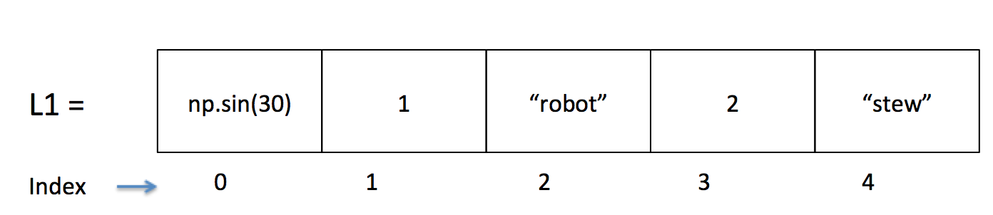
In Python, lists begin by counting with zero. This image below demonstrates a simple list L1, its entries np.sin(30), 1, "robot", 2, "stew", and the corresponding indicies for each entry.

In [10]:

L1 = [np.sin(30), 1, "robot", 2, "stew"]

In [11]:

type(L1)

Out[11]:

list

In [12]:

L1.append(4)

In [13]:

L1

Out[13]:

[-0.98803162409286183, 1, 'robot', 2, 'stew', 4]

In [14]:

L1[1:3]

Out[14]:

[1, 'robot']

In [15]:

L1[2:]

Out[15]:

['robot', 2, 'stew', 4]

In [16]:

L1 * 5

Out[16]:

[-0.98803162409286183,
 1,
 'robot',
 2,
 'stew',
 4,
 -0.98803162409286183,
 1,
 'robot',
 2,
 'stew',
 4,
 -0.98803162409286183,
 1,
 'robot',
 2,
 'stew',
 4,
 -0.98803162409286183,
 1,
 'robot',
 2,
 'stew',
 4,
 -0.98803162409286183,
 1,
 'robot',
 2,
 'stew',
 4]

In [17]:

L1 + L1

Out[17]:

[-0.98803162409286183,
 1,
 'robot',
 2,
 'stew',
 4,
 -0.98803162409286183,
 1,
 'robot',
 2,
 'stew',
 4]

Numpy and Arrays¶

Besides offering some basic numerical operations, numpy has functions built in to generate lists of values. We will use this frequently to construct domains for functions we are investigating. Two functions we will use consistently are the arange and linspace functions. Both are shown below. Remember any NumPy operation will be preceded by np..

In [18]:

np.arange?

In [19]:

np.arange(0, 10, 1)

Out[19]:

array([0, 1, 2, 3, 4, 5, 6, 7, 8, 9])

In [20]:

np.arange(0, 10, 0.5)

Out[20]:

array([ 0. ,  0.5,  1. ,  1.5,  2. ,  2.5,  3. ,  3.5,  4. ,  4.5,  5. ,
        5.5,  6. ,  6.5,  7. ,  7.5,  8. ,  8.5,  9. ,  9.5])

In [21]:

np.linspace?

In [22]:

np.linspace(0, 10, 2)

Out[22]:

array([  0.,  10.])

In [23]:

np.linspace(0, 10, 11)

Out[23]:

array([  0.,   1.,   2.,   3.,   4.,   5.,   6.,   7.,   8.,   9.,  10.])

In [24]:

np.linspace(0, 100, 101)

Out[24]:

array([   0.,    1.,    2.,    3.,    4.,    5.,    6.,    7.,    8.,
          9.,   10.,   11.,   12.,   13.,   14.,   15.,   16.,   17.,
         18.,   19.,   20.,   21.,   22.,   23.,   24.,   25.,   26.,
         27.,   28.,   29.,   30.,   31.,   32.,   33.,   34.,   35.,
         36.,   37.,   38.,   39.,   40.,   41.,   42.,   43.,   44.,
         45.,   46.,   47.,   48.,   49.,   50.,   51.,   52.,   53.,
         54.,   55.,   56.,   57.,   58.,   59.,   60.,   61.,   62.,
         63.,   64.,   65.,   66.,   67.,   68.,   69.,   70.,   71.,
         72.,   73.,   74.,   75.,   76.,   77.,   78.,   79.,   80.,
         81.,   82.,   83.,   84.,   85.,   86.,   87.,   88.,   89.,
         90.,   91.,   92.,   93.,   94.,   95.,   96.,   97.,   98.,
         99.,  100.])

Range¶

The range() function can perform a similar function, however we don’t get an array of values in return. Instead, this simply generates the ability to count through a sequence of integers by a given step. According to the help function, range:

Return an object that produces a sequence of integers from start (inclusive)
to stop (exclusive) by step.  range(i, j) produces i, i+1, i+2, ..., j-1.
start defaults to 0, and stop is omitted!  range(4) produces 0, 1, 2, 3.
These are exactly the valid indices for a list of 4 elements.
When step is given, it specifies the increment (or decrement).

In [25]:

range(10)

Out[25]:

range(0, 10)

In [26]:

range(1, 10, 2)

Out[26]:

range(1, 10, 2)

For Loops and Sequences¶

A for loop defines a repeated series of operations to be carried out a finite number of times. For example, the following code demonstrates the repeated printing of members of range(5).

In [27]:

for i in range(5):
    print(i)

Combining `range`, `for`, and `append`.¶

Together, the for loop, the list, and the ability to add elements to lists with the append function allows us to express repeated operations easily. For example, suppose we want to form a sequence of integers. We can understand this as starting at 1 and adding 1 to each previous term to get the next. Symbolically, we would write this as:

\[a_{i+1} = a_i + 1\]

In Python, we write this as follows.

In [28]:

a = [1]
for i in range(10):
    next = a[i] + 1
    a.append(next)

a

Out[28]:

[1, 2, 3, 4, 5, 6, 7, 8, 9, 10, 11]

Note that the second term is the first element generated within the for loop. We create a variable named next and define it to be the current term of the sequence + 1. We then tack this term on to the end of the list, and continue doing so while i ticks through the values of range(10). Essentially, the loop is building the list piece by piece as follows:

[1]
[1, 2]
[1, 2, 3]
[1, 2, 3, 4]
.
.
.

In [29]:

b = [1]
for i in range(1, 10, 2):
    next = np.sin(i)
    b.append(next)

b

Out[29]:

[1,
 0.8414709848078965,
 0.14112000805986721,
 -0.95892427466313845,
 0.65698659871878906,
 0.41211848524175659]

In [30]:

c = [300]

In [31]:

for i in range(30):
    next = c[i] + 0.03*c[i]
    c.append(next)

c[-5:] #the last five values

Out[31]:

[646.9773802631524,
386701671047,
3783027211784,
9696518028138,
1787413568982]

Functions¶

Most of us have seen functions in high school mathematics. For example, the function

\[f(x) = x^2\]

relates every input to its square. We are quite used to seeing these expressed as plots in a Cartesian coordinate plane. We will deal more with the intricacies of functions through the class, however it is important to be able to define and use basic mathematical functions. For example, to define the function above in Python, we will write:

def f(x):
    return x**2

After doing this, if we want to find the associated value with some input, we can evaluate the function using the parenthesis following its name;

f(3)

We could also evaluate the function for a list of values all at once. Suppose we want to find the value of the first ten integers squared. We can make a list of the ten integers and plug this list into the function rather than evaluating each integer individually.

In [32]:

def f(x):
    return x**2

In [33]:

f(3)

Out[33]:

In [34]:

x = np.arange(1, 11, 1) #first ten integers
f(x)

Out[34]:

array([  1,   4,   9,  16,  25,  36,  49,  64,  81, 100])

Plotting Functions with Matplotlib¶

Often, we can understand a situation better by visualizing it. We will constantly be graphing relationships expressed as function defined as a formula and as a process. Both are demonstrated below using the sequences and functions from above.

First, we tell Jupyter to make the graphs in the notebook itself with the magic command %matplotlib inline. We also import and abbreviate the plotting library PyPlot as plt. Whenever we call something from this library, we preface it with plt..

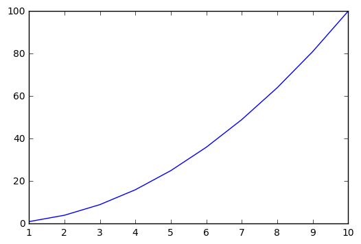
First, we walk through a basic plot of the function \(f(x) = x^2\). We define the function, the \(x\) values we will evaluate it at, and then call the plot with the input and output variables as

plt.plot(x, f(x))

In [35]:

%matplotlib inline
import matplotlib.pyplot as plt

In [36]:

x = np.arange(1, 11, 1)

def f(x):
    return x**2

In [37]:

f(x)

Out[37]:

array([  1,   4,   9,  16,  25,  36,  49,  64,  81, 100])

In [38]:

plt.plot(x, f(x))

Out[38]:

[<matplotlib.lines.Line2D at 0x114f46fd0>]

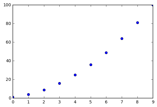
Plotting Sequences with Matplotlib¶

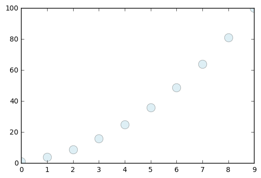
In a similar way, we can generate the plot for a sequence. Because we are interested in the discrete points of the sequence, we will add the marker key o which tells matplotlib to draw circles at each point. The plots can be customized easily, and we then demonstrate altering the size and appearance of the markers as well as how to add titles, labels, and a legend to a plot.

In [39]:

seq = []
for i in range(1,11):
    next = i**2
    seq.append(next)

seq

Out[39]:

[1, 4, 9, 16, 25, 36, 49, 64, 81, 100]

In [40]:

plt.plot(seq, 'o')

Out[40]:

[<matplotlib.lines.Line2D at 0x11555f860>]

In [41]:

plt.plot(seq, 'o', c = 'lightblue', markersize = 12, alpha = 0.4)

Out[41]:

[<matplotlib.lines.Line2D at 0x11568b828>]

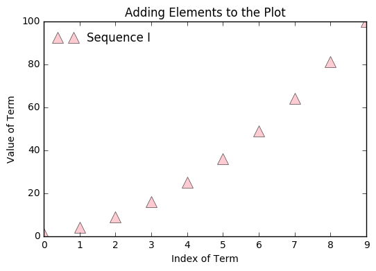
In [42]:

plt.plot(seq, '^', c = 'lightpink', markersize = 12, alpha = 0.7, label = "Sequence I")
plt.title("Adding Elements to the Plot")
plt.xlabel("Index of Term")
plt.ylabel("Value of Term")
plt.legend(loc = "best", frameon = False)

Out[42]:

<matplotlib.legend.Legend at 0x1157afa90>

Sequences and Functions of Import¶

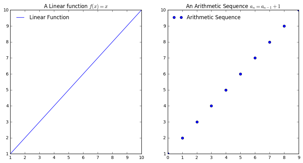
We want to focus on four primary kinds of functions to begin– Linear, Quadratic, Exponential, and Trigonometric. We want to be able to recognize situations that can be modeled by these functions as well as understand the differences between them when expressed as words, numbers, tables, and plots.

We define and plot each as closed functions and as sequences. We introduce the subplot function to place plots side by side. The idea of the subplot function is to declare the number of rows and columns of the figure. For each of these examples we want one row with two columns. Finally, our third value indicates the place of the figure.

plt.subplot(1, 2, 1)

Means 1 row, 2 columns, and place this plot as the first of the two. It should be accompanied by another subplot:

plt.subplot(1, 2, 2)

In [43]:

x = np.linspace(1, 10, 11)
def l(x):
    return x

In [44]:

arith = [1]
for i in range(9):
    next = arith[i] + 1
    arith.append(next)

In [45]:

plt.figure(figsize = (12, 6))
plt.subplot(1, 2, 1)
plt.plot(x, l(x), label = "Linear Function")
plt.title("A Linear function $f(x) = x$")
plt.legend(loc = "best", frameon = False)

plt.subplot(1, 2, 2)
plt.plot(arith, 'o', label = "Arithmetic Sequence")
plt.title("An Arithmetic Sequence $a_n = a_{n-1} + 1$")
plt.legend(loc = "best", frameon = False)

Out[45]:

<matplotlib.legend.Legend at 0x115804630>