In [1]:
%matplotlib inline
import matplotlib.pyplot as plt
import numpy as np
import sympy as sy
Connecting Sums and Differences
We first will discuss some further connections between our earlier work with summations and introduce some problems with differences. We want to note some connections between these operations, and remind ourselves on the important concept of slope.
- Recognize patterns in differences of sequences over small intervals
- Connect patterns in differences to the nature of original sequence
- Determine slope for sequences changing in linear, quadratic, exponential, and trigonometric fashion
First, we will examine some arbitrary sequences. Take, for example the numbers:
First, we want to examine the differences between terms. One way we can do this is similar to our earlier work generating seqences. To start, we will find the difference between 2 and 0, then 6 and 2, then 7 and 4, then 9 and 4. Manually this is easy, but we can also consider this as a list and operate on these numbers based on their index.
In [2]:
f = [0, 2, 6, 7, 4, 9]
In [3]:
f[1], f[0]
Out[3]:
(2, 0)
In [4]:
f[1] - f[0], f[2] - f[1]
Out[4]:
(2, 4)
In the end, we would have the following list \(v\) formed by the subractions starting with index \(i = 0\).
or
We can create this sequence with a for loop.
In [6]:
v = []
n = len(f)
n
for i in range(n-1):
    next = f[i+1] - f[i]
    v.append(next)

v
Out[6]:
[2, 4, 1, -3, 5]
In [7]:
sum(v)
Out[7]:
9
In [8]:
difs = np.diff(f)
difs
Out[8]:
array([ 2, 4, 1, -3, 5])
In [9]:
sum(difs)
Out[9]:
9
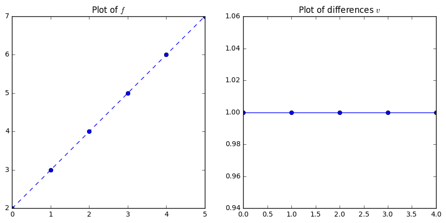
Now let’s examine some more familiar examples of sequences and plot the sequence formed by their difference togethter side by side.
- $ f = 2, 3, 4, 5, 6, 7$
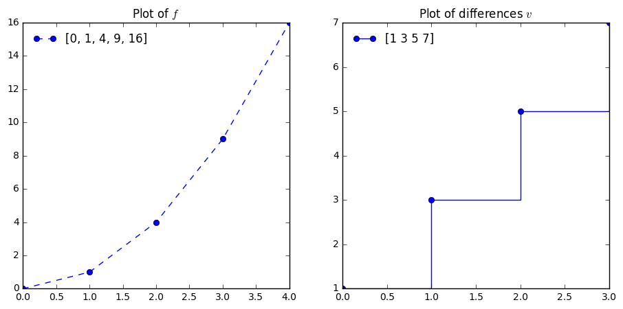
- $ f = 0, 1, 4, 9, 16 $
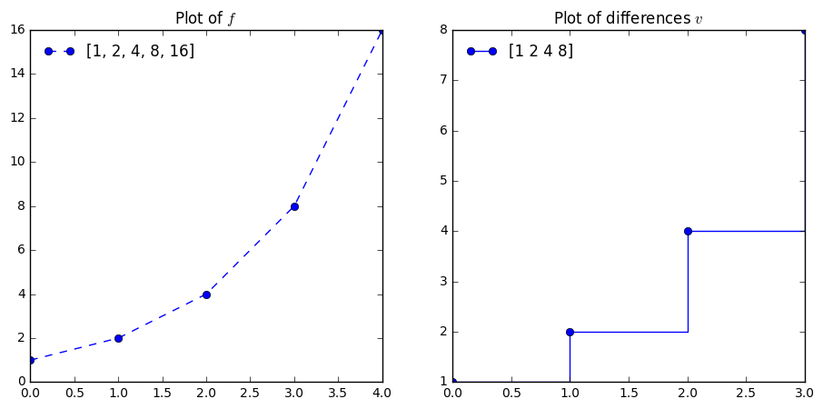
- $ f = 1, 2, 4, 8, 16 $
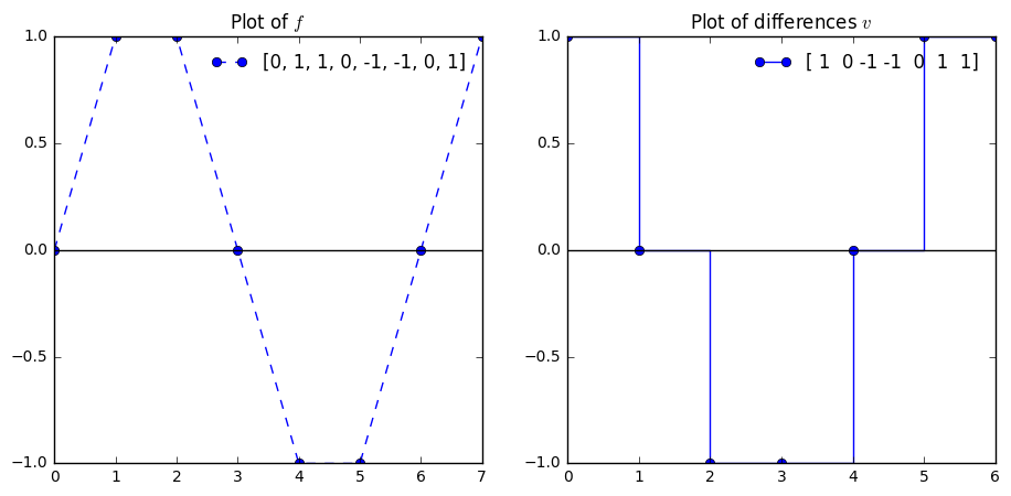
- $ f = 1, 0, -1, -1, 0, 1 $
In [10]:
f = [2, 3, 4, 5, 6, 7]
difs = np.diff(f)

plt.figure(figsize = (11, 5))
plt.subplot(1, 2, 1)
plt.plot(f, '--o')
plt.title("Plot of $f$")

plt.subplot(1, 2, 2)
plt.step(np.arange(len(difs)), difs, '--o', where = 'post')
plt.title("Plot of differences $v$")
Out[10]:
<matplotlib.text.Text at 0x10f83cdd8>
In [11]:
f = [0, 1, 4, 9, 16]
difs = np.diff(f)

plt.figure(figsize = (11, 5))
plt.subplot(1, 2, 1)
plt.plot(f, '--o', label = f)
plt.title("Plot of $f$")
plt.legend(loc = 'best', frameon = False)


plt.subplot(1, 2, 2)
plt.step(np.arange(len(difs)), difs, '--o', where = 'post', label = difs)
plt.title("Plot of differences $v$")
plt.legend(loc = 'best', frameon = False)
Out[11]:
<matplotlib.legend.Legend at 0x1101d1f98>
In [12]:
f = [1, 2, 4, 8, 16]
difs = np.diff(f)

plt.figure(figsize = (11, 5))
plt.subplot(1, 2, 1)
plt.plot(f, '--o', label = f)
plt.title("Plot of $f$")
plt.legend(loc = 'best', frameon = False)


plt.subplot(1, 2, 2)
plt.step(np.arange(len(difs)), difs, '--o', where = 'post', label = difs)
plt.title("Plot of differences $v$")
plt.legend(loc = 'best', frameon = False)
Out[12]:
<matplotlib.legend.Legend at 0x11046ada0>
In [13]:
f = [0, 1,1, 0, -1, -1, 0, 1]
difs = np.diff(f)

plt.figure(figsize = (11, 5))
plt.subplot(1, 2, 1)
plt.plot(f, '--o', label = f)
plt.axhline(color = 'black')
plt.title("Plot of $f$")
plt.legend(loc = 'best', frameon = False)


plt.subplot(1, 2, 2)
plt.step(np.arange(len(difs)), difs, '--o', where = 'post', label = difs)
plt.axhline(color = 'black')
plt.title("Plot of differences $v$")
plt.legend(loc = 'best', frameon = False)
Out[13]:
<matplotlib.legend.Legend at 0x1108dcd30>
Connections to Slope
Recall from high school algebra, the notion of slope as rate of change. If we have two points \((0, 0)\) and \((2, 3)\) and a line between them, we measure the slope of this line as the ratio of change in the vertical direction to that of change in the horizontal direction or:
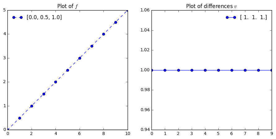
You can verify that the plots on the right side of the figures represent the slope of the line on the left side of the plot. We have also generated plots where the distance between points is a single unit, and can imagine that we would want to move to the the continuous analogies to our sequences above. Let’s start by making plots of twice as many points on the same domains for linear, quadratic, exponential, and trigonometric functions.
In [14]:
f = [i for i in np.arange(0, 5.5, 0.5)]
In [15]:
f
Out[15]:
[0.0, 0.5, 1.0, 1.5, 2.0, 2.5, 3.0, 3.5, 4.0, 4.5, 5.0]
In [16]:
difs = np.diff(f)/0.5
difs
Out[16]:
array([ 1., 1., 1., 1., 1., 1., 1., 1., 1., 1.])
In [17]:
difs/0.5
Out[17]:
array([ 2., 2., 2., 2., 2., 2., 2., 2., 2., 2.])
In [18]:
plt.figure(figsize = (11, 5))
plt.subplot(1, 2, 1)
plt.plot(f, '--o', label = f[0:3])
plt.axhline(color = 'black')
plt.title("Plot of $f$")
plt.legend(loc = 'best', frameon = False)


plt.subplot(1, 2, 2)
plt.step(np.arange(len(difs)), difs, '--o', where = 'post', label = difs[0:3])
plt.title("Plot of differences $v$")
plt.legend(loc = 'best', frameon = False)
Out[18]:
<matplotlib.legend.Legend at 0x110b6ca20>
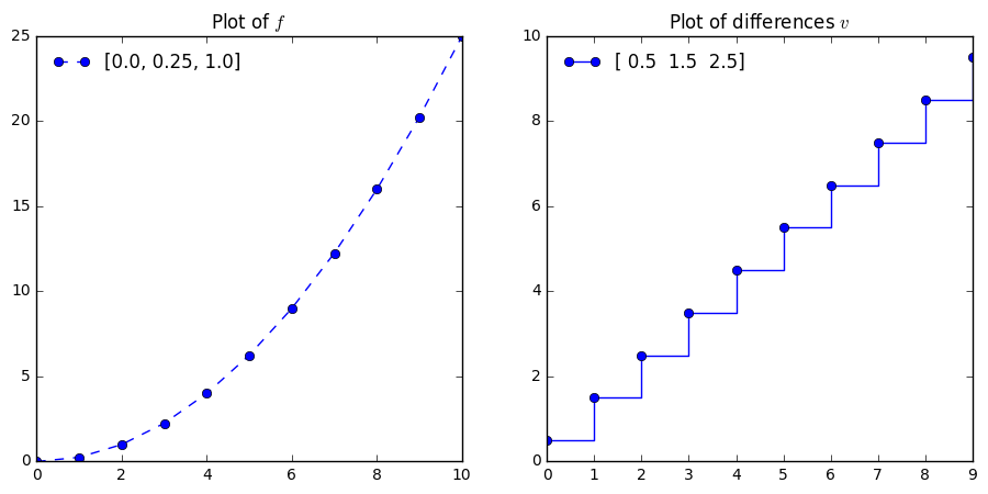
In [19]:
f = [i**2 for i in np.arange(0, 5.5, 0.5)]
In [20]:
difs = np.diff(f)/0.5
In [21]:
plt.figure(figsize = (11, 5))
plt.subplot(1, 2, 1)
plt.plot(f, '--o', label = f[0:3])
plt.title("Plot of $f$")
plt.legend(loc = 'best', frameon = False)


plt.subplot(1, 2, 2)
plt.step(np.arange(len(difs)), difs, '--o', where = 'post', label = difs[0:3])
plt.title("Plot of differences $v$")
plt.legend(loc = 'best', frameon = False)
Out[21]:
<matplotlib.legend.Legend at 0x111004a20>
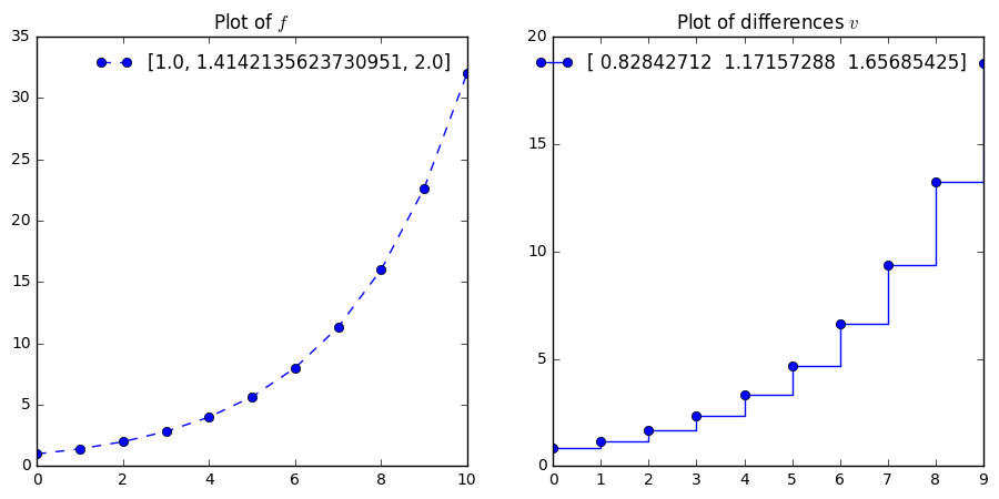
In [22]:
f = [2**i for i in np.arange(0, 5.5, 0.5)]
difs = np.diff(f)/0.5
In [23]:
plt.figure(figsize = (11, 5))
plt.subplot(1, 2, 1)
plt.plot(f, '--o', label = f[0:3])
plt.title("Plot of $f$")
plt.legend(loc = 'best', frameon = False)


plt.subplot(1, 2, 2)
plt.step(np.arange(len(difs)), difs, '--o', where = 'post', label = difs[0:3])
plt.title("Plot of differences $v$")
plt.legend(loc = 'best', frameon = False)
Out[23]:
<matplotlib.legend.Legend at 0x110dce0b8>
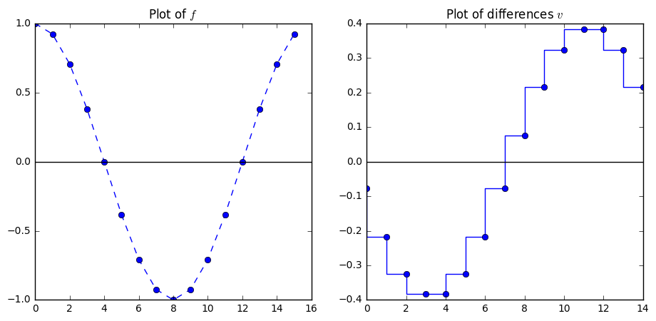
In [24]:
f = [np.cos(i) for i in np.arange(0, 2*np.pi, np.pi/8)]
difs = np.diff(f)

plt.figure(figsize = (11, 5))
plt.subplot(1, 2, 1)
plt.plot(f, '--o')
plt.axhline(color = 'black')
plt.title("Plot of $f$")


plt.subplot(1, 2, 2)
plt.step(np.arange(len(difs)), difs, '--o', where = 'pre')
plt.axhline(color = 'black')
plt.title("Plot of differences $v$")
Out[24]:
<matplotlib.text.Text at 0x1115071d0>
Adding Many Points
We recognize the sequences in closed form for linear, quadratic, exponential, and trigonometric functions here. Remember however, that when we were plotting these functions, we were really just using a large number of points to plug into our function. This means we can still use the plotting instructions from above.
One difference is that we will need to compute the width of the intervals based on how many points we are using. For example, if we use 1000 points on the interval [0, 5], the intervals are each
.
We can divide the entire list of differences by this with the division operation, and we will have our differences to plot. In general, for any interval \([a, b]\) with \(n\) subdivisions, we will have
In [25]:
def f(x):
    return x**2

a = 0
b = 5
n = 1000
w = (b - a)/n

x = np.linspace(a, b, n)
f = f(x)
In [26]:
difs = np.diff(f)/w
In [27]:
plt.figure(figsize = (11, 5))
plt.subplot(1, 2, 1)
plt.plot(f, '--o')
plt.title("Plot of $f$")


plt.subplot(1, 2, 2)
plt.step(np.arange(len(difs)), difs, '--o', where = 'post')
plt.title("Plot of differences $v$")
Out[27]:
<matplotlib.text.Text at 0x1115e74e0>
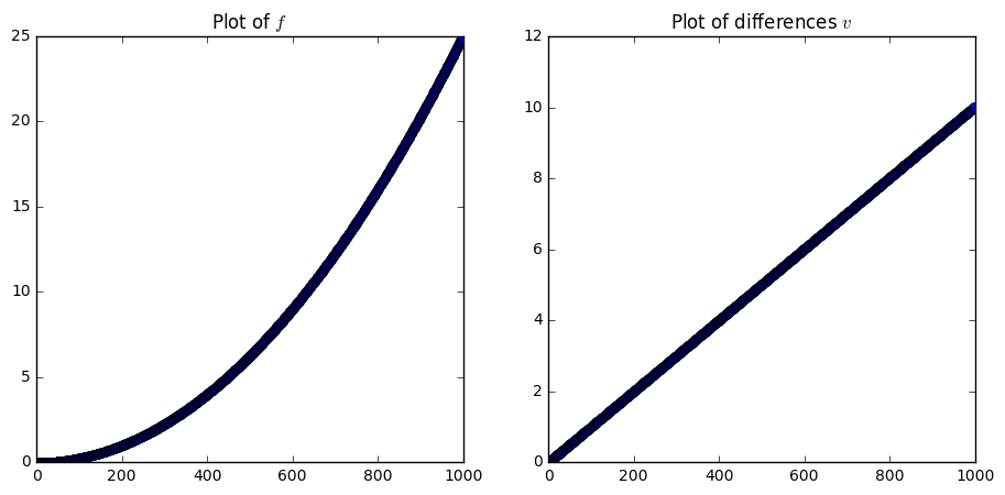
Explore the other examples and see if you can investigate some connections between the kinds of functions \(f\) and its differences \(v\).