In [44]:
%matplotlib inline
import matplotlib.pyplot as plt
import numpy as np
import sympy as sy
Maximum and Minimum Values
Both Pierre de Fermat and G. Wilhelm Leibniz wrote about problems involving maxima and minima of curves. Fermat was interested in the problem of cutting a line so that the product of the length of the resulting segments was maximized.
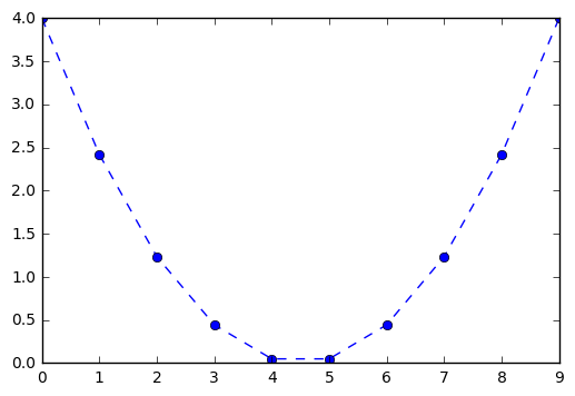
Leibniz was interested in understanding the sign change in differences as a way to notice maximum and minimum values of curves. We follow Leibniz to investigate two simple problems. First, consider sequence \(f_i = i^2\) for \(i\) in \([-2,2]\).
In [45]:
f = [i**2 for i in np.linspace(-2,2,10)]
In [46]:
plt.plot(f, '--o')
Out[46]:
[<matplotlib.lines.Line2D at 0x10d65ab00>]
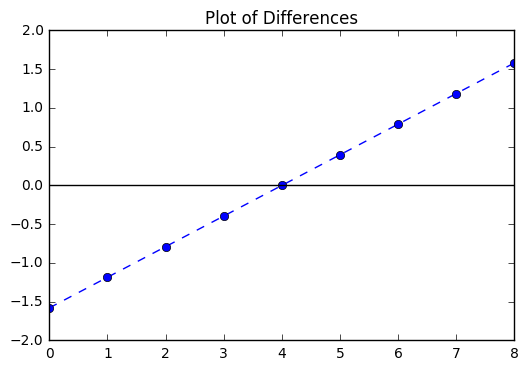
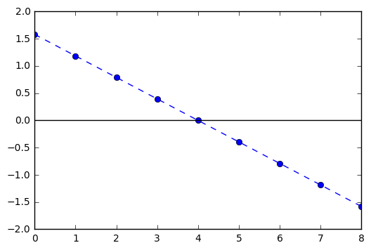
Now, consider the differences of these terms. Recall that we can find
this with the np.diff() function. We also include a horizontal axis
to note the intersection and note something about the connection to
where it seems the minimum value occurs.
In [47]:
diffs = np.diff(f)
In [48]:
plt.plot(diffs, '--o')
plt.axhline(color = 'black')
plt.title("Plot of Differences")
Out[48]:
<matplotlib.text.Text at 0x10d6ad438>
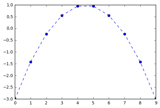
Another example is a similar parabola flipped and pushed up one unit. The result has a maximum value instead of a minimum as we saw in the first example.
In [49]:
f = [-(i**2)+ 1 for i in np.linspace(-2,2,10)]
In [50]:
plt.plot(f, '--o')
Out[50]:
[<matplotlib.lines.Line2D at 0x10d8b7d30>]
In [51]:
diffs = np.diff(f)
In [52]:
plt.plot(diffs, '--o')
plt.axhline(color = 'black')
Out[52]:
<matplotlib.lines.Line2D at 0x10d8d1278>
Smaller Intervals
Let’s suppose we have much smaller intervals between points. For example, suppose we take 100 points on the interval \(x = [-2,2]\). We would be interested in the change between terms, however now this is the number:
In [57]:
def f(x):
    return (x+2) * (x) * (x - 1)
In [58]:
x = np.linspace(-2,2, 100)
dx = (4)/(100)
In [59]:
diffs = np.diff(f(x))/dx
In [68]:
plt.figure(figsize = (11, 6))
plt.subplot(1, 2, 1)
plt.plot(x, f(x), '--o')
plt.axhline(color = 'black')
plt.axvline(color = 'black')
plt.title("Original Function $f(x) = x(x+2)(x-1)$")

plt.subplot(1, 2, 2)
plt.plot(x[1:], diffs, '--o')
plt.axhline(color = 'black')
plt.axvline(color = 'black')
plt.title("Differences in Terms")
Out[68]:
<matplotlib.text.Text at 0x10f69d828>
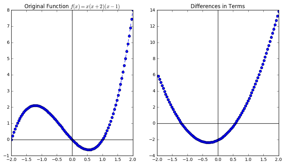
We notice something about the maximum and minimum values, at least locally. When the graph of the function changes direction, the differences are zero. Also, the point considered a local maximum that occurs between \(x = -1.5\) and \(x = -1.0\), the differences change from positive to negative. Similarly for the local minimum near \(x = 0.5\), the differences change from negative to positive.
In [70]:
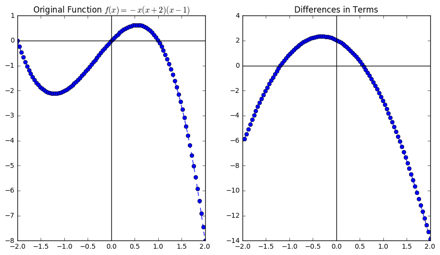
def f(x):
    return -1*(x+2) * (x) * (x - 1)
In [71]:
x = np.linspace(-2,2, 100)
dx = (4)/(100)
diffs = np.diff(f(x))/dx
In [73]:
plt.figure(figsize = (11, 6))
plt.subplot(1, 2, 1)
plt.plot(x, f(x), '--o')
plt.axhline(color = 'black')
plt.axvline(color = 'black')
plt.title("Original Function $f(x) = -x(x+2)(x-1)$")

plt.subplot(1, 2, 2)
plt.plot(x[1:], diffs, '--o')
plt.axhline(color = 'black')
plt.axvline(color = 'black')
plt.title("Differences in Terms")
Out[73]:
<matplotlib.text.Text at 0x10fc3c278>