In [2]:
%matplotlib inline
import numpy as np
import matplotlib.pyplot as plt
import sympy as sy
from sympy import oo
Increasing the Number of Rectangles
In the past examples, we have used rectangles that were fairly wide. This notebook seeks to move from the approximate to the exact case. To do so we relate the idea of summing rectangels to the definition of the definite integral. The video below introduces the big idea of the Riemann integral, which we can understand as an analogous description.
Definite Integral
We can imagine the effect of increasing the number of rectangles to infinity as the ideal way to find the area under the curve. This will be how we introduce the idea of the Definite Integral. The symbol \(\int_a^b\) is used to represent the integral, and \(a\) and \(b\) represent the lower and upper limits for integraion.
For example, the area under the function \(f(x) = x\) from $x = 0 $ to \(x = 1\) would be represented by a definite integral as:
Here, the \(\int_0^1\) tells us we’re summing small little rectangles from \(x = 0\) to \(x=1\). The \(x ~ dx\) represents the area of each rectangle, height \(x\) and infinitely small width \(dx\).
We can solve these problems easily using sympy‘s integrate
function. The function works as follows:
sy.integrate(curve, (variable, start, stop))
The example of \(\int_0^1 x dx\) would be solved as follows.
In [3]:
x = sy.Symbol('x')
sy.integrate(x, (x, 0, 1))
Out[3]:
1/2
Our work to this point is similar to that of a standard definition for an integral from German mathematician Bernhard Riemann. His work took into consideration subdivisions of different widths, and was framed in a much more rigorous manner. Later, in your Real Analysis course, you will formalize the definition and proof of the Reimann integral, but for now we want to recognize situations that we would use a sum
More Curves
Now, let’s suppose that we wanted to find the area under the curve \(g(x) = x^2 + x\) from \(x = -3\) to \(x = 5\). We would represent this with the definite integral:
We can use matplotlib to represent this area with the fill_between
function, and use sympy to evaluate the integral.
In [4]:
def g(x):
    return x**2 + x
In [5]:
x = np.linspace(-3, 5, 1000)
plt.plot(x, g(x))
plt.fill_between(x, g(x), alpha = 0.5)
Out[5]:
<matplotlib.collections.PolyCollection at 0x10d886dd8>
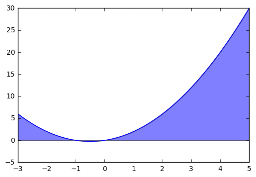
In [6]:
x = sy.Symbol('x')
sy.integrate(g(x), (x, -3, 5))
Out[6]:
176/3
Example II
We want to be comfortable visualizing regions and evaluating the definite integral that represents the area. Let’s represent and find the area under the curve \(y = -3x^3 + 2x + 2\) over the interval \([-2, 1]\).
First, we will plot the curve using matplotlib.
In [8]:
x = np.linspace(-2,1,1000) #create 1000 evenly spaced values from -2 to 1
y = -3*x**3+2*x+2
plt.figure()
plt.plot(x, y, label = '$y=-3x^3 + 2x +2$')
plt.fill_between(x, y, alpha = 0.3, color = 'red', hatch = '|')
plt.legend(frameon=False)
Out[8]:
<matplotlib.legend.Legend at 0x1107a8a20>
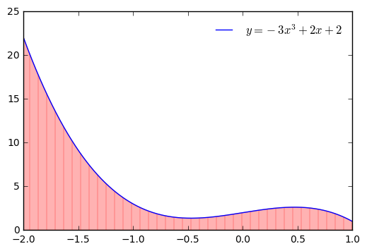
Similarly, we can compute the integral using Sympy.
In [11]:
x, y = sy.symbols('x y')
y = -3*x**3 + 2*x + 2
area = sy.integrate(y, (x, -2,1))
print("The area is: ", area)
The area is: 57/4
We can verify this by hand applying our power rule as follows:
In [14]:
3 + 12 - 4 + 4 -3/4
Out[14]:
14.25