%matplotlib inline
import matplotlib.pyplot as plt
import numpy as np
import sympy as sy

Approximating Values

In this notebook, we approximate solutions to differential equations. This is an important idea, as most differential equations are not easily solved with classical techniques. Our solutions with be numerical values that approximate the exact solutions to the differential equation. Given the initial value problem:

\[\frac{dy}{dx} = 2x + 3 \quad y(0) = 1\]

we want to determine other values of the function near \(x = 0\). To start, we want to consider how to approximate the following values without solving the differential equation, as we already know this is \(y = x^2 + 3x + 1\).

• \(y(0.1)\)
• \(y(0.2)\)
• \(y(0.3)\)
• \(y(1.1)\)

For \(y(0.1)\), consider using the tangent line to approximate this value. We have a line with slope \(2(0.1) + 3 = 3.2\) through the point \((0,1)\). We can write an equation for this line as

\[y = 3.2(x - 0) + 1\]

and investigate this line and the solution around \(x = 0.1\)

plt.figure(figsize = (11,5))
plt.subplot(121)
x = np.linspace(0,0.2,10)
plt.plot(x, x**2 + 3*x + 1, label = 'solution')
plt.plot(x, 3*x + 1, label = 'tangent line')
plt.plot(0.1,1.3,'o', label = '$(0.1, 1.3)$')
plt.legend(loc = 'best')
plt.title('Zooming In around Approximation')

plt.subplot(122)
x = np.linspace(-3,3,100)
plt.plot(x, x**2 + 3*x + 1, label = 'solution')
plt.plot(x, 3*x + 1, label = 'tangent line')
plt.plot(0.1,1.3,'o')
plt.legend(loc = 'best')
plt.title('Zoomed Out view of Approximation')

<matplotlib.text.Text at 0x11312a320>

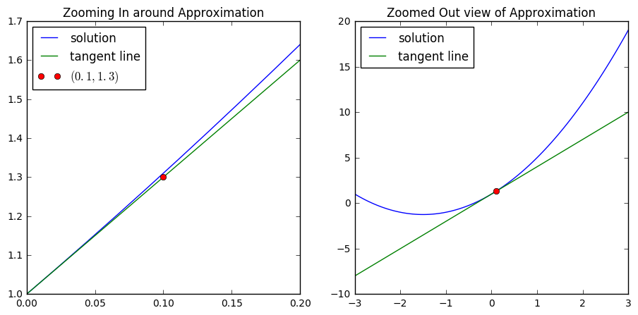
As we notice in the graph on the right, while the tangent line serves as a nice approximation in the near vicinity of our initial value, as we move further away it diverges from the solution.

Euler’s Method

Also, recognize that the differential equation suggests an alternative equation for the tangent line at different \(x\) values. At \(x = 1.1\) the tangent line has a different slope than when \(x=1\). We can adjust every \(0.1\) and write a new equation to traverse for a short period of time. Here, we started at \(x=0\), moved along the tangent line for \(0.1\) units and now write the equation for the tangent line at \(x = 0.1\).

\[y_0 = 1\]

\[tan_1 = (2(0) + 3)(x - 0) + 1 = 3x + 1\]

When \(x=0.1\), we have \(3(0.1) + 1 = 1.3\), so

\[y_1 = 1.3\]

We repeat this process at \((0.1,1.3)\) in order to find \(y_2\).

\[y_2 = (2(0.1) + 3)(0.2 - 0.1)+ 1.3 = 1.62\]

to find \(y_3\) or an approximation for \(y(0.3)\), we simply repeat

\[y_3 = (2(x_2) + 3)(x_3 - x_2) + y_2 = 1.96\]

(2*(0.1) + 3)*(0.2 - 0.1)+ 1.3

1.62

(2*(0.2) + 3)*(0.3 - 0.2)+ 1.62

1.96

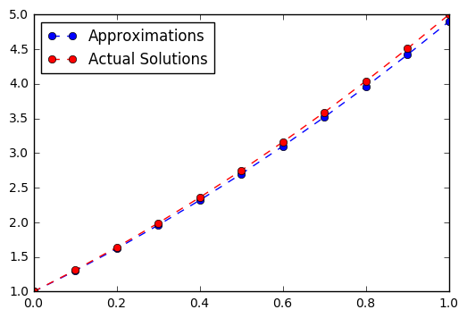
Perhaps you recognize a more general pattern. We are evaluating the derivative at each \(h\) step, multiplying this by \(h\) and adding this to the previous approximation to get our new approximation. Let’s generate more terms and visualize our solutions. Formally, we can define a relationship between successive \(y\) terms as follows, where \(x_i = h*i\) and \(f = \frac{dy}{dx}\):

\[y_{i+1} = h f(x_i) + y_i\]

def df(x):
    return 2*x+3

h = 0.1
y = [1]
for i in range(10):
    next = df(i*h)*h + y[i]
    y.append(next)

y

[1,
 1.3,
 1.62,
 1.9600000000000002,
 2.3200000000000003,
 2.7,
 3.1,
 3.52,
 3.96,
 4.42,
 4.9]

x = np.linspace(0,1.0,11)
plt.plot(x,y,'--o', label = 'Approximations')
plt.plot(x, x**2 + 3*x + 1, '--o', color = 'red', label = 'Actual Solutions')
plt.legend(loc = 'best')

<matplotlib.legend.Legend at 0x113916dd8>

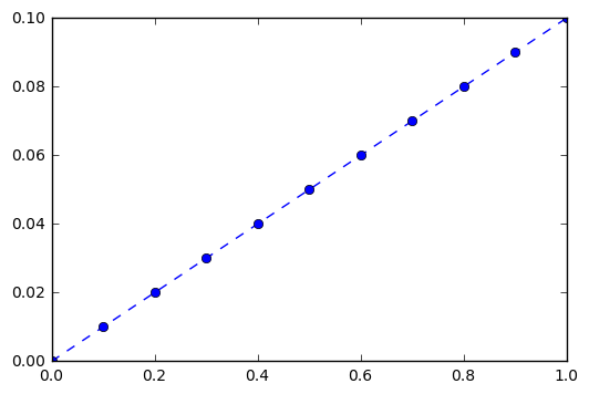
solutions = [(i**2 + 3*i + 1) for i in x]
error = [(solutions[i] - y[i]) for i in range(len(x))]

plt.plot(x, error, '--o')

[<matplotlib.lines.Line2D at 0x113b1e3c8>]

h = 0.01

y2 = [1]
for i in range(100):
    next = df(i*h)*h + y2[i]
    y2.append(next)

x2 = [i for i in np.linspace(0,1.0,101)]
plt.plot(x2, y2, '-k', color = 'red', label = 'Approximation with h = 0.01')
plt.plot(x, y, '--k', color = 'green', label = 'Approximation with h = 0.1')
plt.legend(loc = 'best')

<matplotlib.legend.Legend at 0x113c40b38>

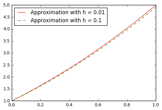
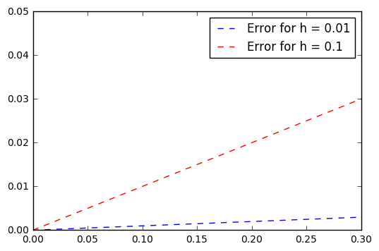
You may not feel this is a big difference, however if we examine the error in these approximations you should notice the divergence in the values depending on the size of \(h\).

solutions2 = [(i**2 + 3*i + 1) for i in np.linspace(0,1,101)]
error2 = [(solutions2[i] - y2[i]) for i in range(100)]
x2 = [i for i in np.linspace(0,1,100)]

plt.plot(x2, error2, '--', color = 'blue', label = 'Error for h = 0.01')
plt.plot(x, error, '--k', color = 'red', label = 'Error for h = 0.1')
plt.legend()
plt.xlim(0,0.3)
plt.ylim(0,0.05)

(0, 0.05)

Population Models

Another familiar differential equation is the exponential growth/decay model. Here, we have a rate of change of a population \(A\) at some time \(t\) for growth rate \(r\) as

\[\frac{dP}{dt} = rP(t)\]

Also, suppose we have the initial condition that at \(t=0\) the population is \(P(0) = 100\), with \(r=2\). Use Euler’s method to approximate solutions at time \(t = .1, .2, .4, 1.1\) with \(h = 0.1, 0.01,\) and \(0.001\). Compare the errors in these approximations to the exact solution to the differential equation.

Populations II

Now suppose we have the differential equation below that models a biological population in time given in hours. Determine an appropriate step size to provide reasonable approximations to the differential equation.

\[\frac{dP}{dt} = 0.003P(t)(2 + 5\sin({\frac{\pi}{12}t})) \quad P(0) = 45000\]

Comparing Exact and Approximates

As mentioned earlier, we cannot always find a function who has a derivative expressed by the differential equation and instead need to use an approximation to find values of a solution. Below, two of the three involve precise solutions. Determine approximations for each, and those that you can find an exact solution using any method please do so.

• \(\frac{dy}{dt} = \cos(t) - y\tan(t) \quad y(0) = 0\)
• \(\frac{dy}{dt} = t\cos(yt) \quad y(0) = 0\)
• \(\frac{dy}{dt} = t^2 \quad y(0) = 0\)