Modeling with Sequences and Functions
A crucial consideration in working with the Calculus is the notion of a rate of change. This notebook aims to familiarize you with four important families of functions and their key characteristics. Next, we present some scenarios where these families serve as appropriate models for particular kinds of situations because of the nature of the quantities change.
Arithmetic Sequences and Linear Functions
An arithmetic sequence is one that exhibits a constant change between terms. Every successive term of the sequence can be determined by multiplication and/or addition by the exact same constant. When plotted, the terms of an arithmetic sequence fall on a straight line.
“In mathematics, an arithmetic progression (AP) or arithmetic sequence is a sequence of numbers such that the difference between the consecutive terms is constant. For instance, the sequence 5, 7, 9, 11, 13, 15, . . . is an arithmetic progression with common difference of 2.” – Wikipedia
In [1]:
arith_1 = [1]
for i in range(5):
    next = arith_1[i] + 1
    arith_1.append(next)

arith_1
Out[1]:
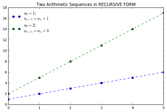
[1, 2, 3, 4, 5, 6]
In [2]:
arith_2 = [2]
for i in range(5):
    next = arith_2[i] +3
    arith_2.append(next)

arith_2
Out[2]:
[2, 5, 8, 11, 14, 17]
In [3]:
%matplotlib inline
import matplotlib.pyplot as plt
import numpy as np
In [4]:
plt.figure(figsize = (8,5))
plt.plot(arith_1, '--o', label = "$a_0 = 1$; \n$a_{n+1} = a_n + 1$")
plt.plot(arith_2, '--o', label = "$a_0 = 2$; \n$a_{n+1} = a_n + 3$")
plt.title("Two Arithmetic Sequences in RECURSIVE FORM")
plt.legend(loc = "best", frameon = False)
Out[4]:
<matplotlib.legend.Legend at 0x10e6b4ac8>
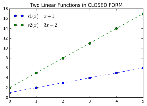
Linear functions exhibit the same behavior. We can recognize linear situations because of a constant rate of change. A linear function is usually defined as:
where \(m\) is the rate of change or slope, and b is the \(y\)-intercept, analagous to \(a_0\) or the starting place in our sequence work. Thus, the sequences above can be defined using our knowledge of the starting value and rate of change (how much is added every term).
We can verify this with a plot.
In [5]:
x = np.arange(0, 6, 1)

def s1(x):
    return x + 1

def s2(x):
    return 3*x + 2

plt.figure()
plt.plot(x, s1(x), '--o', label = '$s1(x) = x + 1$')
plt.plot(x, s2(x), '--o', label = '$s2(x) = 3x + 2$')
plt.title("Two Linear Functions in CLOSED FORM")
plt.legend(loc = "best", frameon = False)
Out[5]:
<matplotlib.legend.Legend at 0x10ef3fa90>
Geometric Sequences and Exponential Functions
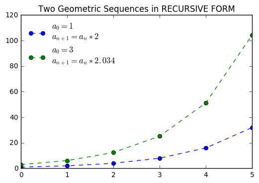
In a Geometric Sequence we generate terms through multiplication.
“In mathematics, a geometric progression, also known as a geometric sequence, is a sequence of numbers where each term after the first is found by multiplying the previous one by a fixed, non-zero number called the common ratio. For example, the sequence 2, 6, 18, 54, ... is a geometric progression with common ratio 3. Similarly 10, 5, 2.5, 1.25, ... is a geometric sequence with common ratio 1/2.”–Wikipedia
The graphs of these sequences exhibit a constant ratio in the rate of change and produce a curve the increases increasingly fast by this multiplier.
In [6]:
geom_1 = [1]
for i in range(5):
    next = geom_1[i]*2
    geom_1.append(next)

geom_1
Out[6]:
[1, 2, 4, 8, 16, 32]
In [7]:
geom_2 = [3]
for i in range(5):
    next = geom_2[i]*2.034
    geom_2.append(next)

geom_2
Out[7]:
[3,
 6.101999999999999,
 12.411467999999998,
 25.244925911999992,
 51.34817930500798,
 104.44219670638623]
In [8]:
plt.figure()
plt.plot(geom_1, '--o', label = "$a_0 = 1$\n$a_{n+1} = a_n *2$")
plt.plot(geom_2, '--o', label = "$a_0 = 3$\n$a_{n+1} = a_n *2.034$")
plt.title("Two Geometric Sequences in RECURSIVE FORM")
plt.legend(loc = "best", frameon = False)
Out[8]:
<matplotlib.legend.Legend at 0x10ed9cdd8>
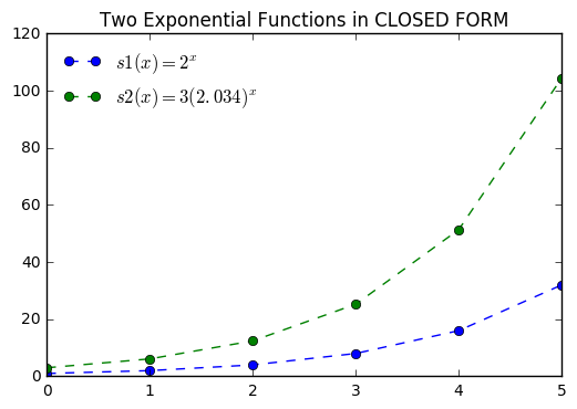
Exponential functions exhibit the same behavior. Typically, exponential functions are defined as:
where \(a\) is analagous to our starting value and \(b\) to the common ration between terms. Thus, we can define the two sequences in closed form as follows:
In [9]:
x = np.arange(0, 6, 1)

def s1(x):
    return 2**x

def s2(x):
    return 3*(2.034)**x

plt.figure()
plt.plot(x, s1(x), '--o', label = '$s1(x) = 2^x$')
plt.plot(x, s2(x), '--o', label = '$s2(x) = 3(2.034)^x$')
plt.title("Two Exponential Functions in CLOSED FORM")
plt.legend(loc = "best", frameon = False)
Out[9]:
<matplotlib.legend.Legend at 0x10f1d0ba8>
Application to Population Growth
A typical application of arithmetic and geometric sequences is to investigate population growth. A very simple model for a population may be:
- Population Model I: Population is currently 500. Every year we add 37 new people.
- Population Model II: Population is currently 500. Every year the population grows by 5.1%.
Model each of these with a recursive sequence and discuss which kind of sequence and closed form is appropriate for each. Then make a side by side plot showing the results of a recursively defined sequence and plot and a closed form function and plot.
Adjusting the Model
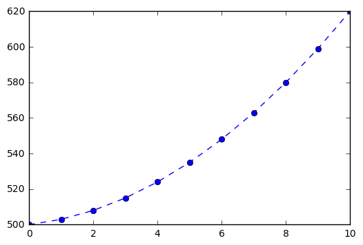
Perhaps the scenarios above seem a little to simplistic. It maybe that rather than changing by the same rate every year, that this rate of change increases as the population grows. If we suppose a constant increase in the rate of change, we are looking at a sequence whose rate of change changes linearly. If we make a sequence whose change is an arithmetic sequence, we should have this.
Note the rate of change between the terms in the sequence below.
In [10]:
p3 = [500]
for i in range(10):
    next = p3[i] + (2*i + 3)
    p3.append(next)

p3
Out[10]:
[500, 503, 508, 515, 524, 535, 548, 563, 580, 599, 620]
In [11]:
plt.plot(p3, '--o')
Out[11]:
[<matplotlib.lines.Line2D at 0x10f31c0b8>]
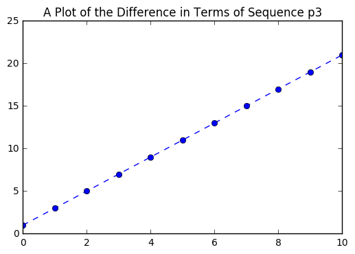
We will return to the closed form of this function later. What is important to notice now is the difference in the way that the sequence is generated. Each term changes by an additively changing amount. We can look closely a the difference in the terms of the sequence.
In [12]:
p3_diff = [1]
for i in range(10):
    next = p3[i+1] - p3[i]
    p3_diff.append(next)
In [13]:
p3_diff
Out[13]:
[1, 3, 5, 7, 9, 11, 13, 15, 17, 19, 21]
In [14]:
plt.plot(p3_diff, '--o')
plt.title("A Plot of the Difference in Terms of Sequence p3")
Out[14]:
<matplotlib.text.Text at 0x10f4f2320>