In [1]:
%matplotlib inline
import matplotlib.pyplot as plt
import numpy as np
import sympy as sy
Composition and the Chain Rule
As you may have guessed, once we apply the idea of differentiation to simple curves, we’d like to use this method in more and more general situations. This notebook explores the use of differentiation and derivatives to explore functions formed by composition, and to use these results to differentiate implicitly defined functions.
GOALS:
- Identify situations where chain rule is of use
- Define and Use Chain Rule
- Use Chain Rule to differentiate implicitly defined functions
- Use Descartes algorithm to explore alternative approach to differentation
Composition of Functions
Functions can be formed by combining other functions through famililar operations. For example, we can consider the polynomial \(h(x) = x^3 + x^2\) as formed by two simpler polynomials \(f(x) = x^3\) and \(g(x) = x^2\) combined through addition. So far, we have not had to worry about this, as differentiation and integration are linear operators that work across addition and subtraction.
If we instead have a function \(h\) given by:
we may recognize the square root function and the polynomial inside of it. This was not formed by addition, subtraction, multiplication, or division of simpler functions however. Instead, we can understand the function \(h\) as formed by composing two functions \(f\) and \(g\) where:
The operation of composition means we apply the function \(f\) to the function \(g\). We would write this as
We can use SymPy to explore a few examples and determine a general rule for differentiating functions formed by compositions. We begin with trying to generalize the situation above, where we compose some function \(g\) into a function \(f\) of the form
It seems reasonable to expect that
You need to adjust this statement to make it true. Consider the following examples, use sympy to differentiate them and determine the remaining terms.
- \((x^2 - 3x)^2\)
- \((x^2 - 3x)^3\)
- \(\sqrt{x^2 - 3x}\)
In [2]:
x = sy.Symbol('x')
y1 = (x**2 - 3*x)**2
y2 = (x**2 - 3*x)**3
y3 = (x**2 - 3*x)**(1/2)
In [3]:
dy1 = sy.diff(y1, x)
sy.factor(dy1)
Out[3]:
2*x*(x - 3)*(2*x - 3)
In [4]:
dy2 = sy.diff(y2, x)
sy.factor(dy2)
Out[4]:
3*x**2*(x - 3)**2*(2*x - 3)
In [5]:
dy3 = sy.diff(y3, x)
dy3
Out[5]:
(1.0*x - 1.5)*(x**2 - 3*x)**(-0.5)
Now consider the examples for \(f(x) = \sin(g(x))\):
- \(\sin{2x}\)
- \(\sin{(\frac{1}{2}x + 3)}\)
- \(\sin{(x^2)}\)
Implicitly Defined Functions
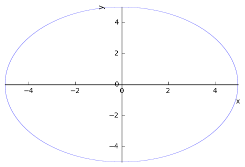
Rather than being given a relationship that can be expressed in terms of a single variable, we can also apply the technique of differentiation to implicitly defined curves. For example, consider the equation for a circle centered at the origin with radius 5, i.e.:
We are unable to express \(y\) in terms of \(x\) with a single equation. We should still be able to understand things like tangent lines however, and apply the idea of differentiation to the expression. We can plot implicitly defined functions with Sympy as shown below. These should look familiar to our parametric plots, and we could introduce parameters into these equations to describe the curves parametrically.
In [6]:
x, y = sy.symbols('x y')
In [7]:
y1 = sy.Eq(x**2 + y**2, 25)
sy.plot_implicit(y1)
Out[7]:
<sympy.plotting.plot.Plot at 0x1144b0780>
In [8]:
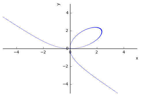
y2 = sy.Eq(x**3 + y**3, (9/2)*x*y)
sy.plot_implicit(y2)
Out[8]:
<sympy.plotting.plot.Plot at 0x1168e74a8>
In [9]:
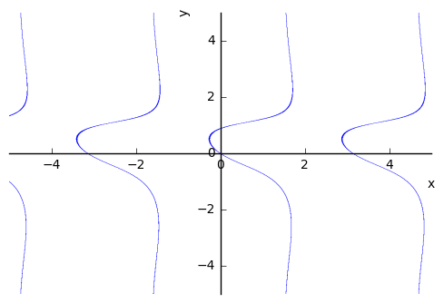
y3 = sy.Eq(sy.sin(x + y), y**2*sy.cos(x))
sy.plot_implicit(y3)
Out[9]:
<sympy.plotting.plot.Plot at 0x1169b3908>
In [10]:
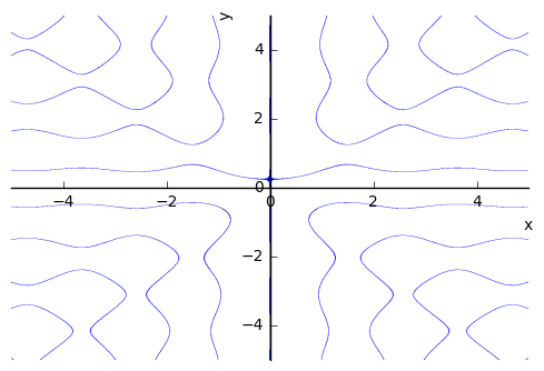
y4 = sy.Eq(y*sy.sin(3*x), x*sy.cos(3*y))
sy.plot_implicit(y4)
Out[10]:
<sympy.plotting.plot.Plot at 0x116a4cef0>
Algorithmic Implicit Differentiation
Hopefully, you recognize the problem. There are many tangents at a given value of \(x\). However, we can determine a point on the graph and recall what we know about equations of lines. Take the second example, called the Folium of Descartes, defined as:
We know the point \((2, 1)\) is on the graph. Also, we know that if we have a tangent line at this point, it would be a linear equation with some slope \(m\) that passes through \((2, 1)\). This means
These equations agree at \((2,1)\) so we can substitute the second into the first for \(y\)
There is some algebra involved here that we will call on Sympy to help us with. Here’s the idea. From the picture, we see there will be two tangent lines at \(x = 2\). This means our equation has a double root there, or that \((x-2)^2\) is a factor of this. We can eliminate one of these roots by dividing the expression by \(x-2\), then substituting \(x=2\) into the remaining expression and solve for the slope \(m\).
In [24]:
x, y, m = sy.symbols('x y m')
expr = x**3 + y**3 -(9/2)*x*y
tan = m*(x-2) + 1
In [25]:
expr = expr.subs(y, tan)
sy.pprint(expr)
 3                                          3
x  - 4.5⋅x⋅(m⋅(x - 2) + 1) + (m⋅(x - 2) + 1)
In [26]:
expr
Out[26]:
x**3 - 4.5*x*(m*(x - 2) + 1) + (m*(x - 2) + 1)**3
In [31]:
now = sy.quo(expr, x-2)
now = now.subs(x, 2)
In [32]:
sy.solve(now, m)
Out[32]:
[1.25000000000000]
Textbook Approach
If we want to work directly on the expression, we can recall that \(y\) can be considered as a function of \(x\), \(y=f(x)\). When we do express things this way, the equation for the Folium above becomes
The left hand side of the equation has the term \(x^3\), whose derivative with respect to \(x\) is \(3x^2\) from our familiar rules, and then our second term, \((f(x))^3\) makes use of the chain rule and we would get:
We treat the other elements of the expression similarly, and solve for
the term \(f'\). We can use Sympy to simplify these computations and
verify the result above. The idiff function from sympy takes the
implicit derivative with respect to the second variable. We can then
evaluate the generale derivative at our point \((2, 1)\).
In [85]:
x, y = sy.symbols('x y')
foli = x**3 + y**3 - (9/2)*x*y
dx_foli = sy.idiff(foli, y, x)
In [86]:
dx_foli.subs(x, 2).subs(y, 1)
Out[86]:
1.25000000000000